안녕하세요? 이번 글은 시리즈 글의 일부로 Google Earth Engine과 geemap을 이용한 종 분포 모델링(SDM: Species Distribution Modeling) 구현 방법을 소개해 보겠습니다. 이 글의 내용은 스미소니언 보전생물연구소 연구진 분들이 제공한 JavaScript 소스코드를 Python으로 변환하여 수정, 보완한 것입니다.
Crego, R. D., Stabach, J. A., & Connette, G. (2022). Implementation of species distribution models in Google Earth Engine. Diversity and Distributions, 28, 904–916. https://doi.org/10.1111/ddi.13491
사례 연구 1: 출현-전용 데이터를 이용한 팔색조(Pitta nympha) 서식지 적합성 및 예측 분포 모델링
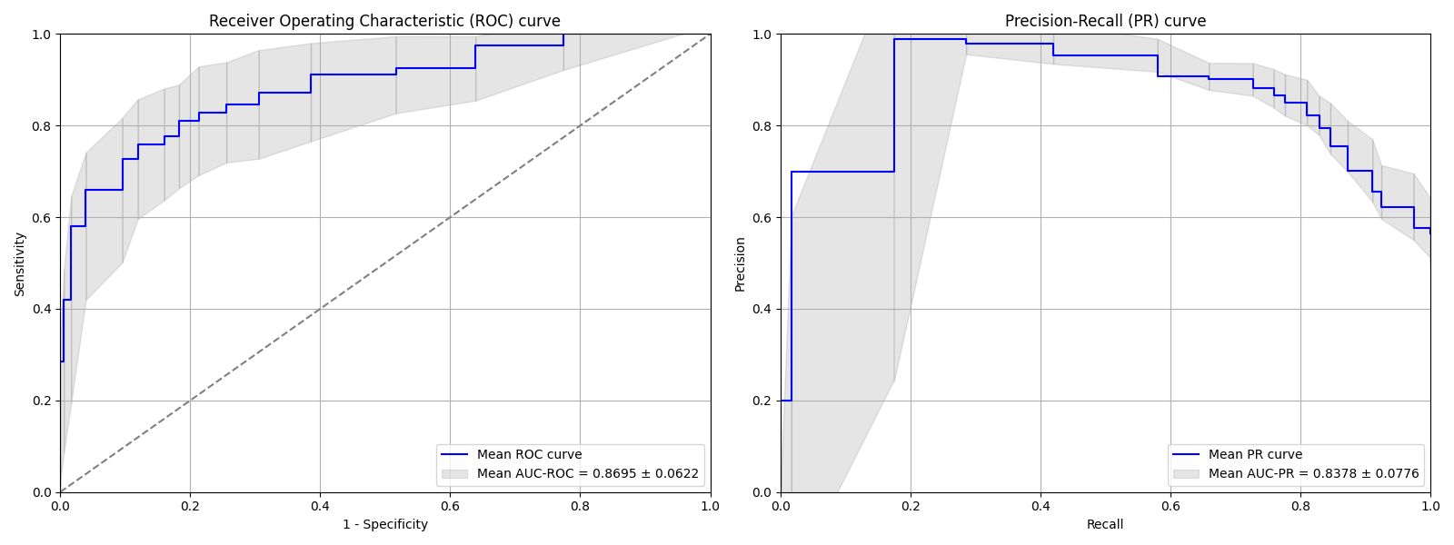
8. 정확도 평가 (ROC PR 곡선 플롯)
이전에 검증 데이터셋을 사용하여 n번의 반복에 대해 AUC-ROC와 AUC-PR를 각각 계산하고 평균과 표준편차를 계산했었는데요, 이를 그래프로 구현하고자 ROC 곡선과 PR 곡선을 추가했습니다. 특히 PR 곡선 관련해서는 아래 논문을 참고해 보시면 좋겠습니다. 일부 내용만 번역 첨부했습니다.
Sofaer, HR, Hoeting, JA, Jarnevich, CS. The area under the precision-recall curve as a performance metric for rare binary events. Methods Ecol Evol. 2019; 10: 565-577. https://doi.org/10.1111/2041-210X.13140
아래 그림은 AUC-ROC 및 AUC-PR 계산에 사용되는 성능 속성을 강조하는 혼동 행렬(confusion matrix)을 나타냅니다.

AUC-ROC는 민감도(Sensitivity, 센시티비티 = Recall) 대 1-특이도(1-Specificity, 스펙시피시티) 그래프 아래의 면적으로, 임계값을 변화시켰을 때의 민감도와 특이도의 관계를 나타냅니다. 민감도는 모든 관측된 비출현에 기반합니다. 따라서 AUC-ROC는 혼동 행렬의 모든 사분면을 포함합니다.
AUC-PR은 정밀도(Precision) 대 재현율(Recall = Sensitivity) 그래프 아래의 면적으로, 임계값을 변화시켰을 때의 정밀도와 재현율의 관계를 나타냅니다. 정밀도는 모든 예측된 출현에 기반합니다. 따라서, AUC-PR은 진음성(TN)의 수를 포함하지 않습니다. AUC-PR을 계산하는데 사용되는 셀은 회색으로 칠해지고 점선으로 윤곽이 그려집니다. TP(True Positive, 진양성); FP(False Positive, 가양성); FN(False Negative, 가음성); TN(True Negative, 진음성)
아래 그림은 (a) ROC(Receiver Operating Characteristic) 곡선과 (b) PR(Precision-Recall) 곡선을 비교한 것입니다. AUC-PR은 출현빈도(low prevalence)가 낮은 희귀종 모델의 평가 및 출현-비출현 클래스의 불균형 상황에서 도움이 되는 것으로 알려져 있습니다.


def plot_roc_pr_curves(images, TestingDatasets, numiter):
    roc_pr_curves = []

    for x in range(numiter):
        HSM = ee.Image(images.get(x))
        TData = ee.FeatureCollection(TestingDatasets.get(x))
        results = getAcc(HSM, TData)

        fpr_values = results.aggregate_array('FPR').getInfo()
        tpr_values = results.aggregate_array('TPR').getInfo()
        precision_values = results.aggregate_array('Precision').getInfo()

        roc_pr_curves.append((fpr_values, tpr_values, precision_values))

    roc_pr_curves_array = np.array(roc_pr_curves)

    fpr_data = roc_pr_curves_array[:, 0]
    tpr_data = roc_pr_curves_array[:, 1]
    precision_data = roc_pr_curves_array[:, 2]

    mean_fpr = np.mean(fpr_data, axis=0)
    mean_tpr = np.mean(tpr_data, axis=0)
    std_fpr = np.std(fpr_data, axis=0)
    std_tpr = np.std(tpr_data, axis=0)
    mean_precision = np.mean(precision_data, axis=0)
    std_precision = np.std(precision_data, axis=0)

    plt.figure(figsize=(16, 6))

    plt.subplot(1, 2, 1)
    plt.step(mean_fpr, mean_tpr, color='b', label='Mean ROC Curve', where='post')
    for i in range(len(mean_fpr) - 1):
        plt.fill_between([mean_fpr[i], mean_fpr[i+1]], [mean_tpr[i] - std_tpr[i], mean_tpr[i+1] - std_tpr[i+1]],
                         [mean_tpr[i] + std_tpr[i], mean_tpr[i+1] + std_tpr[i+1]], color='gray', alpha=0.2)
    plt.plot([0, 1], [0, 1], linestyle='--', color='gray')
    plt.xlim([0, 1])
    plt.ylim([0, 1])
    plt.xlabel('1 - Specificity')
    plt.ylabel('Sensitivity')
    plt.title('Receiver Operating Characteristic (ROC) curve')
    plt.legend(["Mean ROC curve", auc_roc_mean_std], loc='lower right')
    plt.grid(True)

    plt.subplot(1, 2, 2)
    plt.step(mean_tpr, mean_precision, color='b', label='Mean PR Curve', where='post')
    for i in range(len(mean_tpr) - 1):
        plt.fill_between([mean_tpr[i], mean_tpr[i+1]], [mean_precision[i] - std_precision[i], mean_precision[i+1] - std_precision[i+1]],
                         [mean_precision[i] + std_precision[i], mean_precision[i+1] + std_precision[i+1]], color='gray', alpha=0.2)
    plt.xlim([0, 1])
    plt.ylim([0, 1])
    plt.xlabel('Recall')
    plt.ylabel('Precision')
    plt.title('Precision-Recall (PR) curve')
    plt.legend(["Mean PR curve", auc_pr_mean_std], loc='lower right')
    plt.grid(True)

    plt.tight_layout()
    plt.savefig('roc_pr_curves.png')
    plt.show()
%%time
# ROC PR 곡선 플롯
plot_roc_pr_curves(images, TestingDatasets, numiter)